Overview

This sample post teaches you my preferred approach for authoring new posts that need to execute Python code. The post includes a table of contents and code highlighting. The post content covers the use of Conda environments, inserting Python code chunks, and displaying plots.

View the source code on GitHub.

Document metadata

As seen in the source code, the metadata is the information between the --- markers at the top of the source code. Here is where you specify information such as the document author, date, summary, table of contents, code highlighting scheme, tags, and categories.

The metadata for this document contains the following information in the structure shown:

title: Sample post - Using Python in R Markdown
summary: This post shows you how to use Python in an R Markdown document
author: Danny Morris
date: '2021-04-30'
output:
  blogdown::html_page:
    highlight: tango
    toc: true
slug: []
Description: ''
Tags: [Python, Conda, Scikit-Learn]
Categories: [Python, Conda, Scikit-Learn]
DisableComments: no

Activating conda environment

This is optional but highly recommended. Use Conda environments to inform R Markdown of the Python environment you intend to use to execute the Python code in the post. Using either Anaconda or Miniconda, create a conda environment with the libraries needed to run your analysis in Python. Using the reticulate package in R, specify this conda enviornment at the beginning of the document using the use_condaenv() function.

# this is an R chunk
# all other chunks are Python
reticulate::use_condaenv("r-reticulate", required=T)

Load Python packages

import numpy as np
import matplotlib.pyplot as plt
from sklearn.ensemble import IsolationForest

Fit isolation forest

rng = np.random.RandomState(42)

# Generate train data
X = 0.3 * rng.randn(100, 2)
X_train = np.r_[X + 2, X - 2]
# Generate some regular novel observations
X = 0.3 * rng.randn(20, 2)
X_test = np.r_[X + 2, X - 2]
# Generate some abnormal novel observations
X_outliers = rng.uniform(low=-4, high=4, size=(20, 2))

# fit the model
clf = IsolationForest(max_samples=100, random_state=rng)
clf.fit(X_train)

## IsolationForest(max_samples=100,
##                 random_state=RandomState(MT19937) at 0x7D2B1505DD40)

Predict outliers

y_pred_train = clf.predict(X_train)
y_pred_test = clf.predict(X_test)
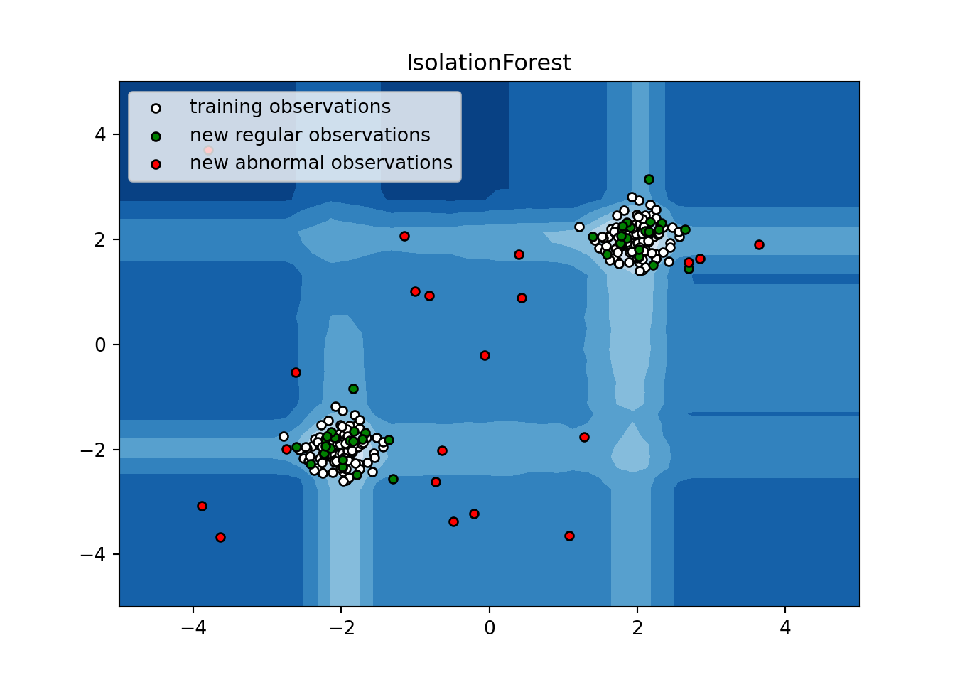
y_pred_outliers = clf.predict(X_outliers)

Plot outliers

# plot the line, the samples, and the nearest vectors to the plane
xx, yy = np.meshgrid(np.linspace(-5, 5, 50), np.linspace(-5, 5, 50))
Z = clf.decision_function(np.c_[xx.ravel(), yy.ravel()])
Z = Z.reshape(xx.shape)

plt.title("IsolationForest")
plt.contourf(xx, yy, Z, cmap=plt.cm.Blues_r)

## <matplotlib.contour.QuadContourSet object at 0x7d2b0fdce1c0>

b1 = plt.scatter(X_train[:, 0], X_train[:, 1], c='white',
                 s=20, edgecolor='k')
b2 = plt.scatter(X_test[:, 0], X_test[:, 1], c='green',
                 s=20, edgecolor='k')
c = plt.scatter(X_outliers[:, 0], X_outliers[:, 1], c='red',
                s=20, edgecolor='k')
plt.axis('tight')

## (-5.0, 5.0, -5.0, 5.0)

plt.xlim((-5, 5))

## (-5.0, 5.0)

plt.ylim((-5, 5))

## (-5.0, 5.0)

plt.legend([b1, b2, c],
           ["training observations",
            "new regular observations", "new abnormal observations"],
           loc="upper left")
plt.show()